Sign in to Guacamole
Guacamole displays a CAE Linux desktop in your browser. The tools run on the CAE machine. Use your own UW NetID and confirm that your account can reach CAE Linux services before the lab.
- On your laptop, open https://guacamole.cae.wisc.edu in a browser.
- Complete the UW web sign-in with your NetID and password, then complete MFA if requested.
- At the Linux login screen, enter your UW NetID and password again. Use your NetID credentials at this second prompt too. The old separate CAE username and password are not the instructions for this service.
- Wait for the Linux desktop. Open Apps in the upper-left corner and choose Terminal under Favorites. Maximize the terminal by double-clicking its title bar.
- Keep the Guacamole tab open. A terminal inside this desktop is already on CAE; do not SSH back into CAE from it.
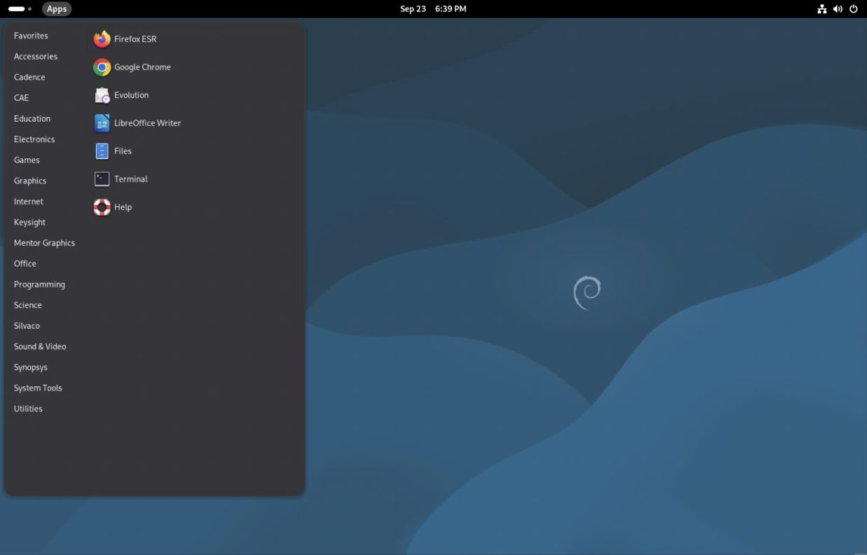
If you already have an active session, the browser may reconnect without showing every login screen. If sign-in fails, record which prompt failed: UW web sign-in, MFA, or the Linux desktop login. These are different stages.
More help with Guacamole sign-in, including CAE's official instructions and screenshots: https://kb.wisc.edu/cae/163323
Enter the Synopsys environment
Run these commands in the CAE terminal, one line at a time. Do not type a prompt such as $ or synopsys> before a command.
module load synopsys/suite
synopsys-run
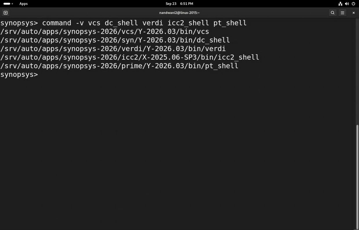
command -v vcs dc_shell verdi icc2_shell pt_shell
The prompt becomes synopsys>. The module selects the site setup; the container provides the operating environment expected by the tools. Load the module before entering the container and repeat this setup for every new terminal used for Synopsys tools.
Companion code
RTL: https://github.com/abhinavnandwani/cae-synopsys-guides/blob/main/lab/rtl/sb_flop.v
Testbench: https://github.com/abhinavnandwani/cae-synopsys-guides/blob/main/lab/tb/tb.sv
Simulation runner: https://github.com/abhinavnandwani/cae-synopsys-guides/blob/main/lab/run_lab.py
Commands below use ~/cae-synopsys-guides/lab as the exercise directory. The recorded screenshots show the original dated demonstration folder.
Work confidently in the terminal
The current directory affects relative paths. pwd prints it, ls lists files, cd .. moves to the parent, and cd ~/cae-synopsys-guides/lab returns to the exercise. A leading / means an absolute path; ~ means your home directory. Quote paths containing spaces.
| Prompt or location | Commands that belong there |
|---|---|
| Laptop Terminal or PowerShell | ssh to reach the CAE host shell. |
| CAE host shell | module load synopsys/suite, then synopsys-run. |
Container synopsys> | Linux commands, python3 run_lab.py, vcs, verdi, dc_shell, and icc2_shell. |
Tool prompt such as dc_shell> | Tool Tcl commands such as read_ddc, report_timing, and help. |
Use these from the exercise folder to inspect source and logs without changing them:
ls -lh
cat rtl/sb_flop.v
sed -n '1,80p' tb/tb.sv
less runs/YOUR_RUN/compile.log
grep -nE 'Error|Fatal|Warning' runs/YOUR_RUN/compile.log
tail -n 30 runs/YOUR_RUN/simulate.log
Replace YOUR_RUN with an actual directory printed by the runner. In less, use Space to advance, /Error then Enter to search, n for the next match, and q to return to the shell. An Up-arrow recalls a command; Tab completes a path. Read a command before rerunning it.
For an interactive foreground command that is stuck, Ctrl+C requests interruption. For a GUI launched with &, close the application through its File menu. jobs lists jobs started by that shell. Keep logs: command > run.log 2>&1 sends both standard output and errors to a file. Immediately after a command, echo $? reports its exit status, but a zero status alone does not prove the design passed.
Connect without the browser when useful
For terminal-only work, open a terminal on your laptop and run ssh YOUR_NETID@best-tux.cae.wisc.edu, then load the module and enter the container as above. Use Guacamole for the GUI steps in this handout. SSH and Guacamole may reach different hosts, but your CAE home directory is shared.
When finished, save work, close the EDA applications, and run exit to leave the container. Log out of the Linux desktop from the upper-right system menu. Closing the browser alone can leave the session running during CAE's two-hour reconnection window.
Run the verification exercise from the terminal
Inside the Synopsys container, start from the companion folder:
cd ~/cae-synopsys-guides/lab
python3 run_lab.py simulation
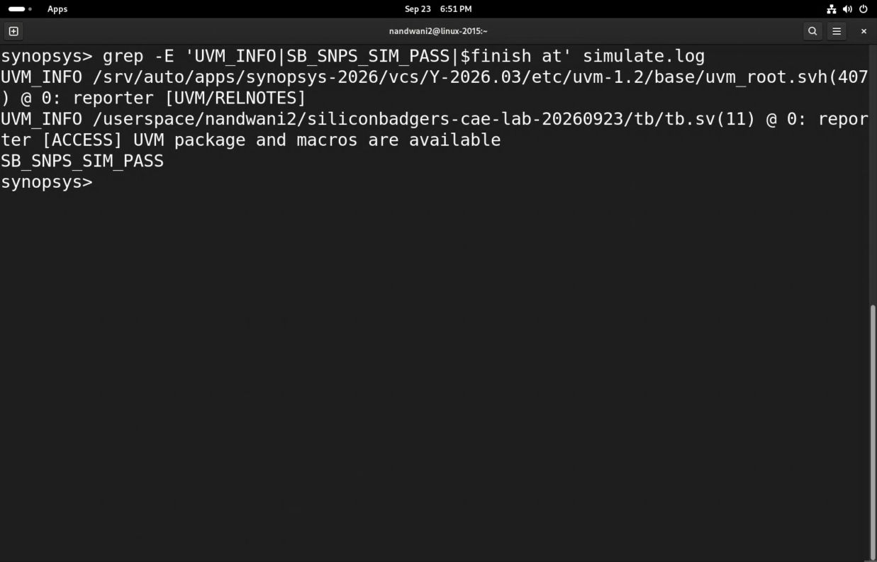
The runner creates a new directory under runs/ for every invocation. It compiles the design, executes a passing simulation, builds a coverage report, and executes a separate intentionally failing simulation. The final LAB_RESULT=PASS means these checks behaved as expected, including detection of the deliberate failure.
| File in the printed run directory | How to use it |
|---|---|
compile.log | Start here for syntax, missing include, package, and elaboration errors. |
simulate.log | Inspect test diagnostics, simulation time, and the pass marker. |
simv | The compiled simulation executable for this build. |
smoke.fsdb | Waveform data for the passing run. |
simv.vdb | Collected coverage data. |
coverage_report/ | URG's HTML coverage report. |
negative/expected_failure.log | Evidence that the injected fault was detected. |
result.json | Exact commands, working directories, elapsed time, raw exit codes, and verdict. |
Change into the exact run directory the runner printed. Do not guess that an older directory is the latest run. Inspect result.json and the logs even when the final result says PASS. A working test harness and a correct design are separate questions.
Understand and reproduce the terminal commands
The example has rtl/sb_flop.v and tb/tb.sv. The testbench instantiates the register, drives a 10 ns clock, checks reset, checks captured data, and writes an FSDB. UVM 1.2 is imported to check that the installed integration works; this example is a procedural testbench, not a complete class-based UVM environment.
To run the commands directly, create a separate manual run directory first:
SB_LAB="$HOME/cae-synopsys-guides/lab"
SB_RUN=$(mktemp -d "$SB_LAB/runs/manual-sim-XXXXXX")
cd "$SB_RUN"
export VERDI_HOME="$(dirname "$(dirname "$(command -v verdi)")")"
vcs -full64 -sverilog -timescale=1ns/1ps \
  -ntb_opts uvm-1.2 -debug_access+all -kdb \
  -cm line+cond+tgl+branch+assert \
  "$SB_LAB/rtl/sb_flop.v" "$SB_LAB/tb/tb.sv" \
  -top tb -o simv > compile.log 2>&1
echo $?
./simv -cm line+cond+tgl+branch+assert > simulate.log 2>&1
grep -nE 'Error|Fatal|SB_SNPS_SIM_PASS' simulate.log
urg -full64 -dir simv.vdb -report coverage_report \
  > coverage.log 2>&1
Stop after compilation if it fails. The shell does not automatically stop this sequence for you. The supplied Python runner is preferable for repeatable runs because it checks diagnostics and required outputs and gives each command a 180-second limit.
-full64 selects the working 64-bit VCS mode on this installation. -sverilog enables SystemVerilog parsing. -top tb selects the testbench top. -debug_access+all -kdb retains information needed for source-level debugging. The -cm options enable the listed coverage types; they do not create missing assertions or functional coverage goals.
Inspect the test before trusting it
Read the checks in tb/tb.sv. At 11 ns the test checks the reset value and drives one onto d. It checks q at 21 ns, then drives zero. It checks again at 31 ns. These checks occur after the relevant rising edge so the nonblocking assignment has completed. A real interface test should define its sampling convention just as explicitly.
Open Verdi and navigate the design
From the passing simulation directory, launch the GUI inside Guacamole:
verdi -ssf smoke.fsdbKeep that terminal available for launch diagnostics. Maximize Verdi by double-clicking its title bar. The hierarchy pane identifies instances; the source pane shows their code; the lower nWave pane displays recorded signal values.
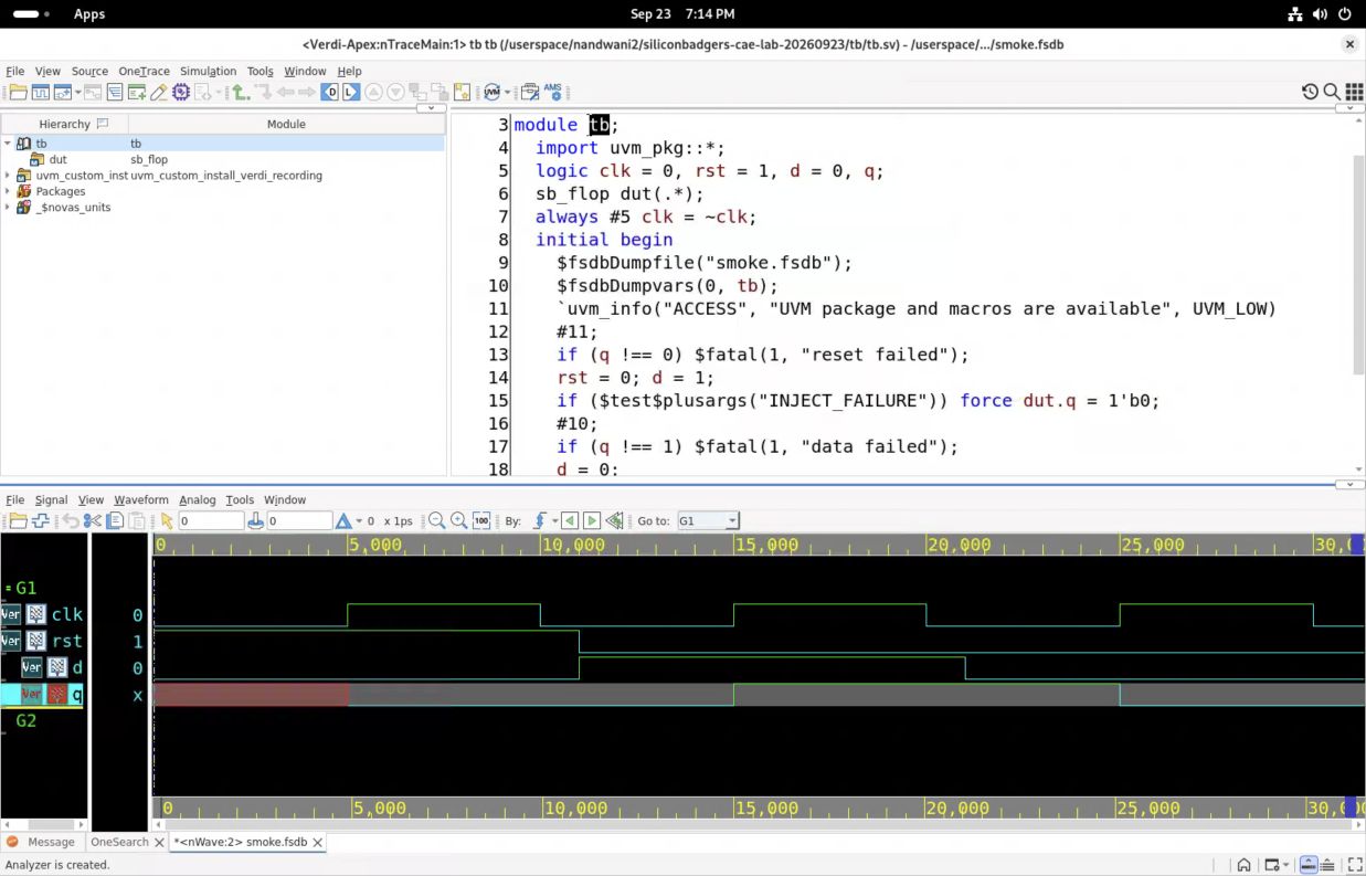
- In the hierarchy pane, select
tb. Expand it and selectdutto inspect the instantiatedsb_flopmodule. Confirm that you opened the intended source and top. - Return to
tbto read the stimulus and checks alongside the RTL. Locate the clock generator, reset release, assignments tod, and$fatalchecks. - In the lower nWave pane, choose Signal, then Get Signals. Select the
/tbscope in the dialog. - Select
clk,rst,d, andq. In the tested interface, selecting a signal and clicking Apply adds it to the waveform list. Repeat for the four signals, then click OK. - In nWave, choose View, then Zoom, then Zoom All. This displays the entire saved simulation rather than just its initial few nanoseconds.
If the source view is empty, first confirm that you launched from the run directory that contains the matching build data. Do not mix one build's debug database with another build's waveform. If the waveform list is empty, adding signals is still required even though the FSDB loaded successfully.
Debug the waveform rather than just displaying it
Start with all four signals visible and the full 0 to 31 ns interval. The recorded view uses picoseconds on the ruler: 10000 ps is 10 ns. Signal values in the value column correspond to the current cursor position, not necessarily the end of the run.
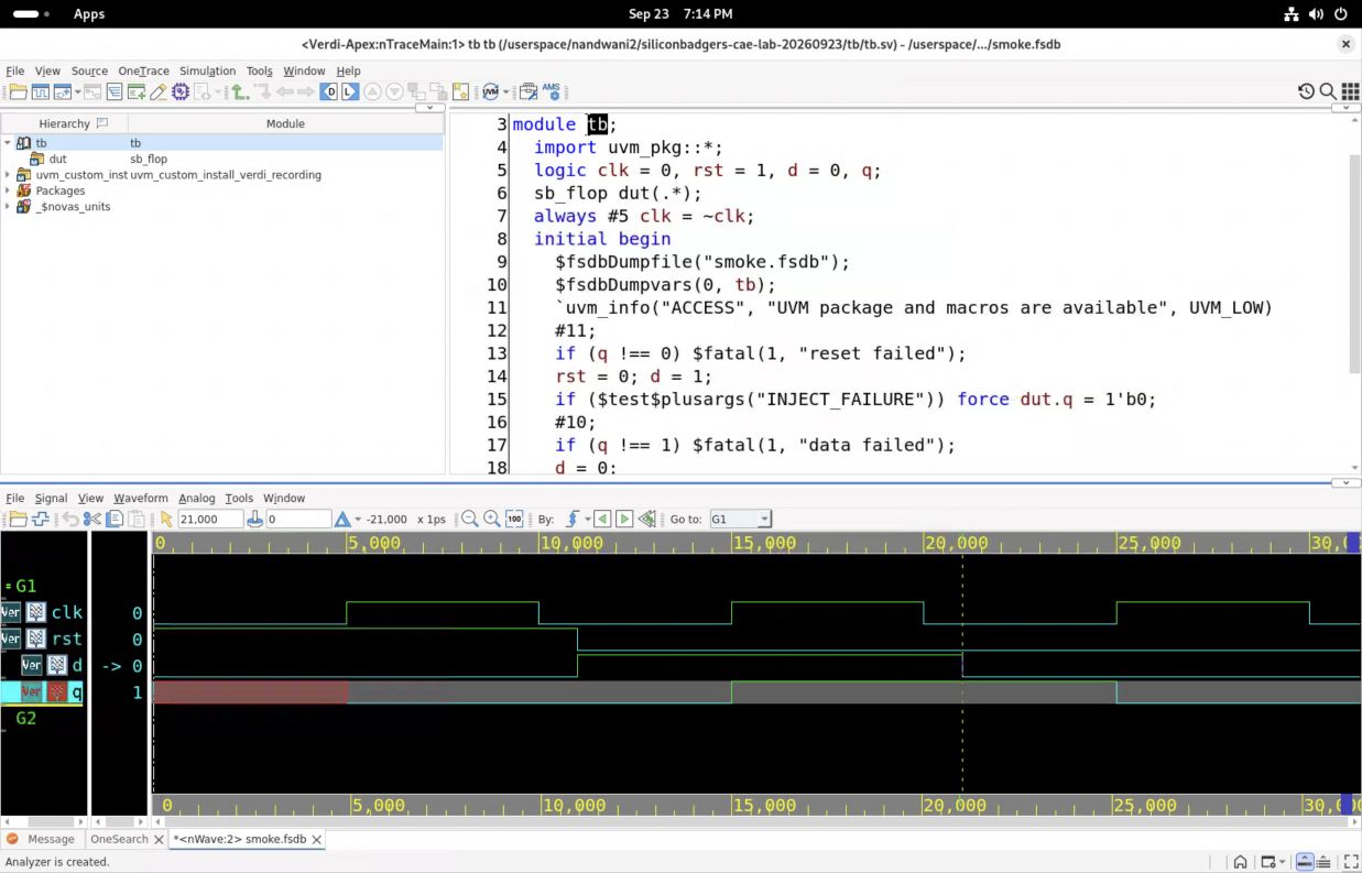
- Click in the waveform near the first rising edge of
clk. Follow the same vertical time position throughrst,d, andq. - Move the time cursor before and after the edge. Before the first rising edge,
qis unknown. At 5 ns, the asserted synchronous reset sets it to zero. - Inspect the reset release and data change at 11 ns. The output should not update immediately because the register samples on the next rising edge.
- Inspect 15 ns.
qcaptures one. Inspect 21 ns whendreturns to zero, then 25 ns whenqcaptures zero. - Use the nWave View, Zoom menu to inspect a smaller interval, then Zoom All to recover the overview. Keep the clock visible when investigating a data transition.
| Time | Expected observation |
|---|---|
| Before 5 ns | q is unknown; no active clock edge has applied reset yet. |
| 5 ns | q becomes zero while rst is high. |
| 11 ns | rst becomes zero and d becomes one. |
| 15 ns | q becomes one. |
| 21 ns | d becomes zero. |
| 25 ns | q becomes zero. |
| 31 ns | Final check completes and simulation ends. |
Write down the first time observed behavior differs from expected behavior. Then return to the source driving or sampling that signal. A waveform file existing proves only that recording worked; the test's checks and these transitions establish the example's behavior.
Save the signal arrangement with nWave File, Save Signal. Give the file a descriptive .rc name in the run directory. Use File, Restore Signal to load that arrangement in a later session with the matching FSDB. This saves a view configuration, not new simulation results. For readable screenshots, enlarge Monospaced Font under Tools, Preferences, General, Appearance.
Investigate the deliberately failing run
The runner invokes the simulation again with +INJECT_FAILURE in a separate negative/ directory. At 11 ns, the test forces the register output to zero. The expected one is therefore missing at the 21 ns check.
cat negative/expected_failure.log
verdi -ssf negative/smoke.fsdb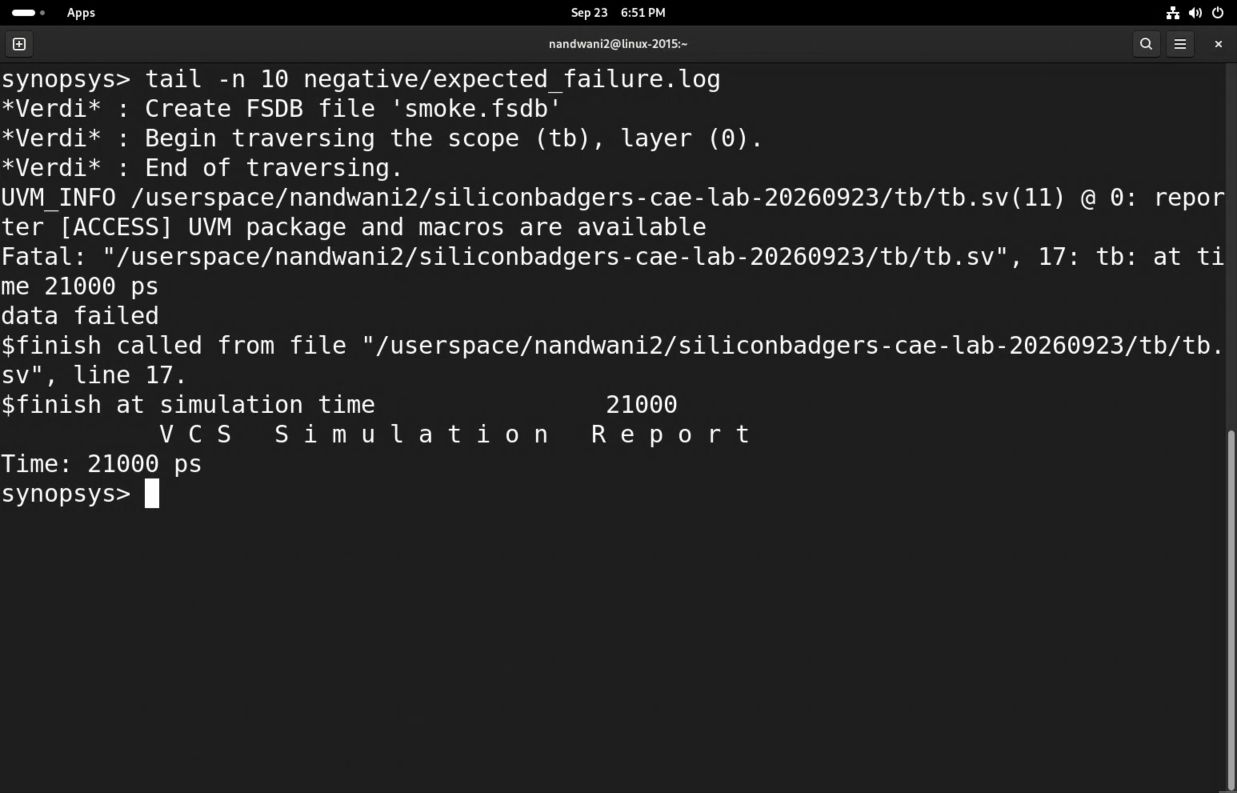
In the failing waveform, add the same four signals. Confirm that d becomes one but q stays zero, then locate the failed check at 21 ns in the source. Compare against the passing run at 15 ns and 21 ns. A separate viewer is useful for comparing the two results; close each viewer when finished.
On the tested installation, VCS returned raw exit code zero even for this fatal diagnostic. The runner therefore requires the positive pass marker, rejects unexpected error or fatal diagnostics, and separately verifies that the deliberate failure reports data failed without the pass marker. Do not use exit zero as the only test verdict.
Preserve both sides of the comparison
Keep the passing and failing logs and waveforms in their separate directories. Record the expected failure text and time. When adapting this pattern, inject a fault that violates a specific requirement and confirm that the intended checker catches it. A crash during compilation is not evidence that a behavioral checker works.
Inspect coverage in the GUI
In the CAE desktop file manager, open the passing run's coverage_report folder and open dashboard.html with Firefox. Alternatively, in a CAE host terminal, run firefox /absolute/path/to/coverage_report/dashboard.html. This browser runs on CAE; the file is not on your laptop.
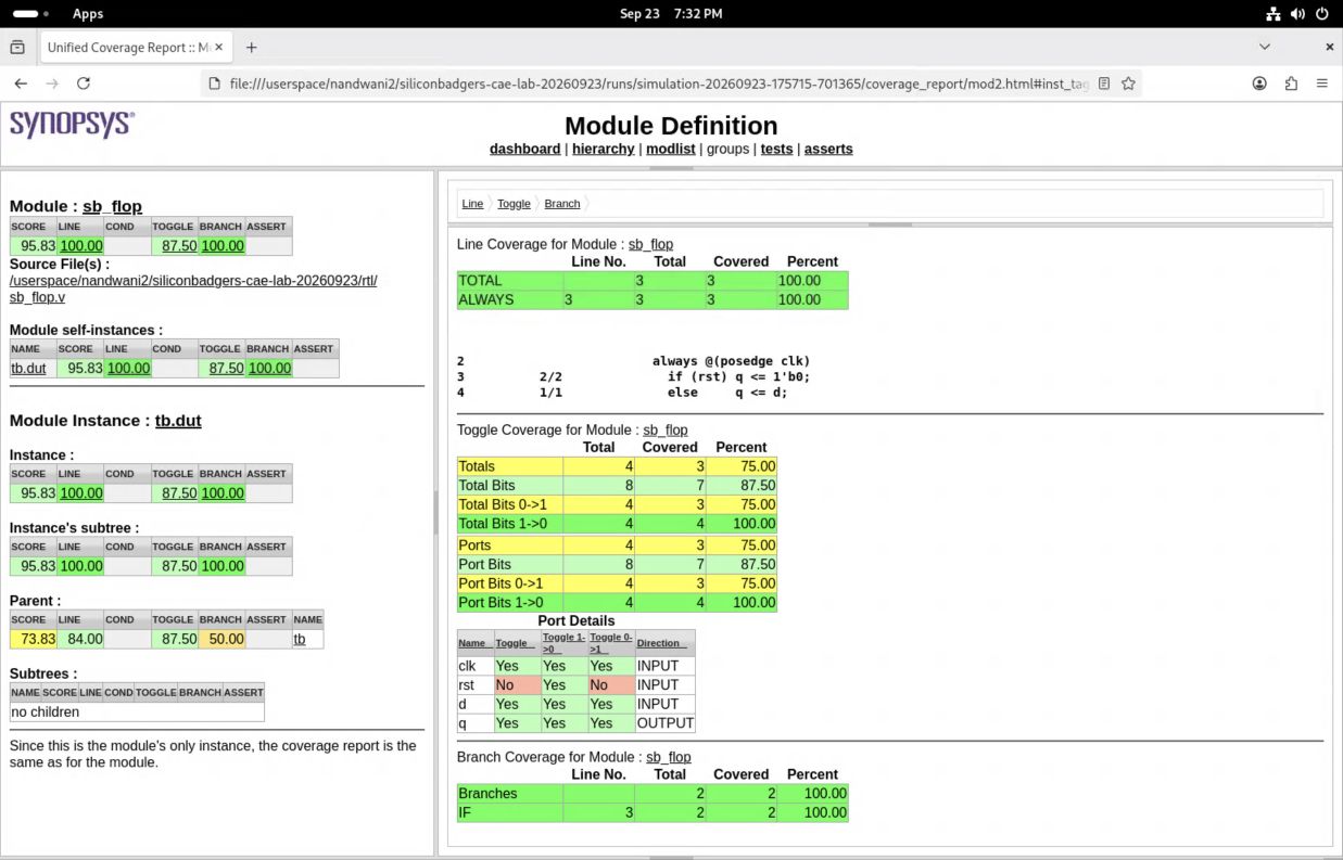
- On the dashboard, check the run date, tool version, command line, and test count. This example report contains one passing test; the deliberately failing run is separate.
- Click hierarchy at the top. Expand
tbif necessary, then click itsdutchild. The module page should identifysb_flopand the instancetb.dut. - Inspect Line and Branch. The tested DUT shows 100% for both. Match the covered source statements to the reset and data paths in the RTL.
- Inspect Toggle and its Port Details table. The DUT reports 87.5% toggle coverage.
rsthas a falling transition but no rising transition because the test starts in reset and never reasserts it. - Compare the DUT with the dashboard totals. The totals also include testbench and imported UVM code. Always record the measured scope and metric with a percentage.
As a follow-on exercise, reassert reset after capturing data, check the resulting output at the appropriate clock edge, and regenerate the report in a fresh run. Confirm both the new behavior and the previously missing transition. Increasing coverage without a meaningful check is not sufficient.
Condition and assertion coverage do not have meaningful DUT targets in this tiny example. High code coverage does not establish arithmetic correctness, protocol behavior, corner cases, or interactions between units.
Reproduce a saved simulation
Keep the source and run files together so you can investigate a result later. These records help distinguish a source change from a tool or configuration difference.
| What a runnable test should retain | Why it is needed |
|---|---|
| Source revision and source manifest | Identifies the exact implementation and test compiled. |
| Tool version and full commands | Makes setup and build differences diagnosable. |
| Seed and configuration when applicable | Reproduces randomized or configurable behavior. |
| Timeout and explicit verdict | Distinguishes a hang, a crash, and a failed check. |
| Logs, waveform, and coverage | Preserves evidence for debugging and review. |
| Known failing case | Shows that the checker rejects incorrect behavior. |
Troubleshoot in a consistent order
If compilation fails, read the first relevant error before investigating later errors that may be consequences. Check the top module, source list, package and include order, and SystemVerilog flags. If simulation starts but no pass marker appears, inspect where it stops and whether the expected checker ran. If the GUI is blank, check the selected FSDB, scope, signal list, and matching build directory.
If a tool prints only a CAE launcher warning, return to the host shell and load the module before entering the container. For a license failure, retain the exact diagnostic and tool version. For an unresponsive GUI, first allow startup or loading to complete; do not repeatedly start duplicate copies that each consume resources.
Check your setup
The passing run should contain SB_SNPS_SIM_PASS; the deliberately failing run should contain data failed without that pass marker. In Verdi, compare the reset and data transitions with the table above. In URG, check which reset transition is missing from toggle coverage.
Tested on CAE with VCS Y-2026.03_Full64, Verdi Y-2026.03, and URG Y-2026.03. Setup reference: https://kb.wisc.edu/cae-software-guide
Verdi overview: https://www.synopsys.com/verification/debug/verdi.html